A Practical Guide on How to Calculate Terminal Value

To get to a company's total value, you have to look beyond the next five or ten years. That's where Terminal Value comes in. It’s a single number that represents all of a company's expected future cash flows from the end of your forecast period into eternity.

You've got two main ways to figure this out: the Perpetuity Growth Method, which assumes the company grows at a steady, slow pace forever, and the Exit Multiple Method, which estimates what someone might pay for the business down the road. This isn't just a minor calculation—it often makes up the vast majority of a company's total value in a Discounted Cash Flow (DCF) model.

What Is Terminal Value and Why It Matters in DCF

Let's be realistic: trying to forecast a company's financials year-by-year for the next 50 years is a fool's errand. The uncertainty becomes massive. That's why in finance, we typically build detailed projections for a manageable period, usually five to ten years.

But what about all the years after that? That's the exact problem terminal value solves. It's a single, calculated estimate of a company's worth for every year beyond the explicit forecast period, assuming it hits a stable, mature phase.

A DCF model without terminal value would be like telling a story and stopping halfway through. It would ignore a huge chunk of the company's long-term potential.

Here’s why it's so critical:

• It Captures Long-Term Worth: A healthy company doesn't just shut down after year five. Terminal value puts a number on its ability to keep generating cash far into the future.

• It Simplifies the Impossible: Instead of making hundreds of impossible annual guesses, it uses a single, stable growth assumption to represent the company's entire future from that point on.

• It Carries the Most Weight: This might be surprising, but for mature companies, terminal value often accounts for 70-90% of the total enterprise value in a DCF. This means your assumptions here have a massive impact on the final number. You can find more great insights on this at mccrackenalliance.com.

Key Takeaway: Think of a DCF valuation in two parts. Part one is the detailed, year-by-year forecast for the next 5-10 years. Part two, the terminal value, is a snapshot representing the company's value from that point forward, forever.

The Two Trusted Calculation Methods

So, how do you actually calculate this all-important number? Finance pros lean on two well-established methods. Each one comes at the problem from a slightly different angle, giving you a different perspective on the company's long-term value.

Comparing the Two Core Methods for Calculating Terminal Value

Here's a quick comparison of the Perpetuity Growth and Exit Multiple methods, outlining their core logic, key inputs, and ideal scenarios for use.

As you can see, the Perpetuity Growth Method (also called the Gordon Growth Model) is an intrinsic approach. It’s perfect for businesses that have hit their stride and are expected to grow predictably, like a major utility or a blue-chip consumer goods company.

The Exit Multiple Method, on the other hand, is all about market perception. It's the go-to for analyses where a sale is the likely outcome, like in a private equity or M&A context.

Choosing which one to use isn't just about plugging in numbers; it's a strategic decision. You have to think about the company's industry, where it is in its lifecycle, and what you're actually trying to accomplish with your valuation.

Calculating Terminal Value With The Perpetuity Growth Method

This is the classic, most common way to calculate terminal value. The Perpetuity Growth Method, also known as the Gordon Growth Model, is built on a simple idea: eventually, a company matures and its cash flows will grow at a slow, steady rate forever.

It's an intrinsic approach, meaning it values the company based on its own long-term ability to generate cash.

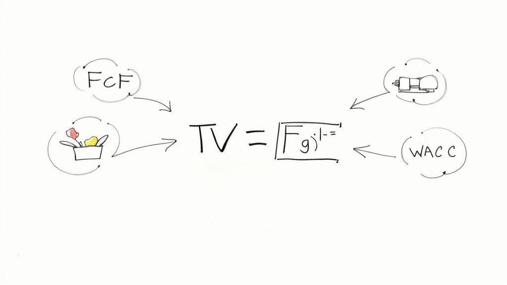
The formula itself looks deceptively simple. The real art is in defending your assumptions.

Terminal Value (TV) = [FCFn * (1 + g)] / (WACC - g)

Let's break down what each of these inputs actually means in the real world.

What Goes Into the Formula?

Every variable in this model tells a piece of the company's story. Getting them right is the difference between a real valuation and a random number.

• FCFn (Final Year Free Cash Flow): This is the free cash flow from the very last year of your detailed forecast (say, Year 5 or Year 10). Think of it as the launchpad for all future cash flows.

• g (Perpetual Growth Rate): The constant rate you expect the company’s cash flow to grow forever. This is, without a doubt, the most debated input in any DCF model.

• WACC (Weighted Average Cost of Capital): This is your discount rate. It’s what you use to pull all those future dollars back to what they're worth today, reflecting the risk of the investment.

The top part of the formula, FCFn * (1 + g), is just calculating the cash flow for the first year after your forecast ends. The bottom, (WACC - g), is the "capitalization rate"—it's the magic number that turns that single year of cash flow into the total value for every year after that, forever.

Choosing Your Starting Cash Flow

Your FCFn isn't just a number you pull from your spreadsheet. It has to represent a "normalized" year for the business.

If the last year of your forecast includes a massive, one-time factory expansion or a huge working capital swing, using that number will throw off your entire valuation. It needs to reflect a steady state.

For example, with a mature manufacturing company, you want the FCF to reflect routine maintenance capex, not a once-in-a-decade facility overhaul.

Pro Tip: If your final forecast year's FCF looks wonky, try averaging the FCF from the last two or three years of the forecast. This helps smooth out any noise and gives you a more reliable baseline for perpetuity.

Nailing Down a Defensible Growth Rate

The perpetual growth rate, g, is where people get into trouble. It's easy to be optimistic, but this number has to be tethered to reality. A company simply cannot grow faster than the entire economy forever.

The most common rookie mistake is setting 'g' too high. For a company in a developed economy like the U.S., a defensible growth rate is typically between 2% and 3%. This aligns with long-term GDP growth or inflation targets, which is a key best practice explained by valuation experts at McCracken Alliance.

Here are a few guardrails for picking 'g':

• GDP Growth: The long-term growth rate of the economy where the company operates is the ultimate ceiling for 'g'.

• Inflation: At the very least, a stable company should grow in line with inflation just to maintain its real value.

• Company Size: Huge, mature companies (think Coca-Cola) should have a 'g' closer to or even below GDP growth.

And here's a critical mathematical check: 'g' must always be less than your WACC. If it's not, the formula spits out a negative or infinite number, which is a flashing red light that your assumptions are impossible.

A Quick Practical Example

Let’s run the numbers for a hypothetical company, "Sturdy Steel Inc."

After building our 5-year DCF model, we land on these assumptions:

• Final Year FCF (FCF₅): $50 million

• Perpetual Growth Rate (g): 2.5% (we're pegging this to expected long-term GDP growth)

• Weighted Average Cost of Capital (WACC): 8.0%

Now, just plug and chug.

1. First, calculate the cash flow for Year 6 (the first year of perpetuity): $50 million * (1 + 0.025) = $51.25 million

2. Next, find the capitalization rate: 8.0% - 2.5% = 5.5%

3. Finally, divide to get the Terminal Value: $51.25 million / 0.055 = $931.82 million

So, the Terminal Value of Sturdy Steel at the end of Year 5 is roughly $932 million. This single number represents the value of every single cash flow from Year 6 into the distant future. The next step would be to discount this value back to today and add it to the present value of the forecast-period cash flows.

Using the Exit Multiple Method for Valuation

While the perpetuity method is all about a company's internal cash flow, the Exit Multiple Method flips the script. It looks outward and asks a much more practical question: "If we sold this business at the end of the forecast, what would a real buyer actually pay for it?"

This approach calculates terminal value by assuming the company is sold for a multiple of a key financial metric. The formula itself is dead simple:

Terminal Value (TV) = Financial Metric x Exit Multiple

The real art isn't in the math; it's in picking the right metric and defending your multiple. This method is grounded in market reality, which is why it's a favorite among private equity and M&A folks who are always thinking about the eventual exit.

Selecting the Right Financial Metric

The "Financial Metric" in the formula is the engine of your whole calculation. Your choice here hinges entirely on the company's industry, maturity, and profitability. You have to pick a metric that buyers in that specific market are actually using to value businesses today.

Here are the most common choices and the logic behind them:

• EBITDA (Earnings Before Interest, Taxes, Depreciation, and Amortization): This is the workhorse for most mature, stable companies. EBITDA serves as a proxy for operating cash flow and isn't skewed by accounting choices like depreciation, making it perfect for comparing companies with different capital structures.

• EBIT (Earnings Before Interest and Taxes): This gets used more in industries where capex is a big deal, like manufacturing or utilities. Because it subtracts depreciation, it offers a more conservative view of profitability than EBITDA.

• Revenue: For high-growth, early-stage companies (think tech or SaaS), profits might be low or even negative. In these cases, investors value the business on a multiple of its revenue, essentially betting on future profitability.

Picking the wrong metric can make your valuation look completely out of touch. You wouldn't value a pre-profit biotech startup on its EBITDA, just like you wouldn't value a 100-year-old railroad only on its revenue.

Finding and Justifying Your Exit Multiple

This is where you put on your detective hat. The exit multiple isn't a number you just make up; it's a reflection of current market sentiment. Your job is to find out what multiples similar companies are trading at or were recently bought for.

Your two main sources will be:

1. Comparable Public Companies ("Public Comps"): Look at publicly traded companies in the same industry with similar size, growth, and risk profiles. Financial data platforms will show you their current trading multiples (e.g., Enterprise Value / LTM EBITDA).

2. Precedent Transactions ("M&A Comps"): This involves analyzing recent M&A deals in the industry. This data is incredibly powerful because it shows you the exact multiples that buyers have actually paid to acquire similar companies.

Crucial Insight: Precedent transaction multiples are often seen as more relevant. They reflect what a strategic buyer—who might pay a premium for control and synergies—is willing to shell out. Trading multiples, on the other hand, just reflect what public market investors will pay for a minority stake.

The quality of your comparable data is everything. For instance, if you were valuing a software company in 2023, you might find that an EV/EBITDA multiple of 12.0x is the average from recent M&A deals in that specific SaaS sub-sector. Using that number ensures your valuation is anchored in reality.

Applying the Method to a Tech Startup

Let's make this real. Imagine we're valuing "InnovateTech," a growing B2B SaaS company. We've already built a 5-year financial model and now we need to figure out its terminal value.

Here are our assumptions for the final year of the forecast:

• Final Forecast Year (Year 5) EBITDA: $25 million

• Selected Metric: EBITDA makes sense. InnovateTech is mature enough now to be consistently profitable.

• Chosen Exit Multiple: After digging into recent acquisitions of similar SaaS companies, we found that buyers were paying an average of 14.0x EV/EBITDA.

Now, we just plug it into the formula:

Terminal Value = Final Year EBITDA x Exit Multiple

Terminal Value = $25 million x 14.0 = $350 million

The calculation is easy, but the story you tell is what sells it. We can now confidently say that, based on current M&A market conditions, InnovateTech could reasonably be sold for $350 million at the end of our forecast period.

This market-based approach often feels more tangible and provides a solid "reality check" against the more theoretical perpetuity growth model. For anyone prepping for finance interviews, being able to walk through this logic is critical. You can practice this and other scenarios with our detailed guide on investment banking case studies. This kind of hands-on prep is exactly what interviewers are looking for.

From Future Value to Today's Worth: Bringing It All Together

So you’ve calculated the terminal value. Great. That’s a huge milestone, but remember what that number actually represents: the company's worth at some point in the future—say, five years from now.

And since a dollar tomorrow is worth less than a dollar today, you need to pull that future value back to what it’s worth right now. We call this discounting.

The formula for this is pretty straightforward:

Present Value of Terminal Value (PV of TV) = TV / (1 + WACC)^n

This just takes your terminal value (TV) and discounts it using the Weighted Average Cost of Capital (WACC) over the number of years in your forecast (n). For a typical five-year model, n is 5.

What’s the Discount Factor All About?

That denominator, (1 + WACC)^n, is what we call the "discount factor." It’s just a way of quantifying the time value of money and the risk baked into those future cash flows.

Think of it this way: the higher the risk (WACC) and the further out you go (n), the less that future value is worth to you today.

For example, if you have a 5-year forecast and a 10% WACC, your discount factor is (1.10)^5, which comes out to roughly 1.61. This means a terminal value calculated for the end of year 5 is worth about 62% less in today’s dollars. It's a steep haircut, but it accurately reflects the risk and time involved.

This visual shows how the Exit Multiple method gets you to that initial terminal value before you even start discounting.

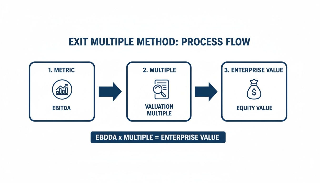
It boils down to three key things: picking the right financial metric, finding a multiple you can defend, and then doing the math to get that future value.

Finishing the Puzzle: Calculating Enterprise Value

Once you have the present value of your terminal value, you’re on the home stretch. The company's total value, or its Enterprise Value, is just the sum of two parts:

1. The Present Value of Forecasted Cash Flows: This is the sum of all the discounted cash flows from your explicit forecast period (e.g., Years 1 through 5).

2. The Present Value of the Terminal Value: This is the single number you just calculated, which represents the value of all cash flows beyond that forecast period.

Enterprise Value = (PV of Forecast Period FCFs) + (PV of Terminal Value)

By adding these two together, you’ve successfully bridged the gap between the company's near-term performance and its long-term potential, all in today's dollars. This final number is what your entire analysis has been building toward—a single figure representing the company’s intrinsic value.

Of course, all of this hinges on a solid grasp of how the financials link together. If you feel shaky on that, our guide on walking through the 3 financial statements is the perfect place to shore up your foundation.

Common Pitfalls and How to Build a Defensible Model

Calculating terminal value can feel like a precise science, but it's really more of an art form built on defensible assumptions. Getting this part wrong can torch your entire valuation, no matter how perfect your five-year forecast is. The biggest mistakes usually come from small judgment calls that snowball into major credibility problems.

These aren't just math errors; they're logic errors. An overly optimistic growth rate or mismatched multiples can make an entire DCF model look amateurish. The goal isn't to find one "correct" number. It's to build a model that can stand up to scrutiny and tell a believable long-term story about the company.

The Overly Optimistic Growth Rate

The most common trap with the Perpetuity Growth Method is setting the perpetual growth rate (g) too high. It's easy to assume a company will keep growing at a solid clip, but "in perpetuity" is an incredibly long time.

A company simply cannot outgrow the economy forever. If it did, it would eventually become the economy. Your perpetual growth rate needs to be anchored to a long-term, macroeconomic benchmark.

• The Golden Rule: The growth rate must be lower than the long-term nominal GDP growth rate of the country where the company primarily operates. For a U.S.-based company, this almost always means a rate between 2.0% and 3.0%.

• Inflation as a Floor: At a minimum, a stable company should be able to grow at the rate of inflation just to maintain its real value. This often serves as a logical floor for your assumption.

Pushing your growth rate above these conservative benchmarks requires an extraordinary explanation. You'd have to build a bulletproof case that the company has a near-permanent competitive advantage allowing it to consistently outpace the market for decades to come. It’s a tough sell.

Mismatched Multiples and Metrics

When you're using the Exit Multiple Method, the real danger is applying the wrong multiple to your final year's financial metric. This is less about calculation and more about common sense and context.

You wouldn't use a high-growth SaaS company's EV/Revenue multiple for a mature industrial manufacturer. The market values these businesses on entirely different drivers, so doing so is a fundamental mismatch that immediately calls your analysis into question.

Sanity Check: Ask yourself, "Would a real-world buyer today actually pay this multiple for this kind of business?" If the answer is no, your multiple is wrong. Always pull your multiples from a carefully curated peer group of companies with similar growth profiles, margins, and risk.

The Double-Counting Growth Error

A more subtle but equally dangerous mistake is double-counting growth. This happens when you take a terminal free cash flow (FCF) from a high-growth forecast period and then slap a healthy perpetual growth rate on top of it.

Your final forecast year should represent a "normalized" or steady-state year. If your capex is artificially low or your working capital improvements are unsustainable in that final year, you're baking aggressive growth into your FCF base. Adding another growth rate on top of that just inflates the valuation with assumptions you can't defend.

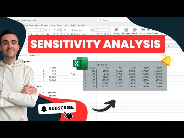
The Ultimate Defense: Sensitivity Analysis

Let's be honest: your assumptions are educated guesses. The best way to handle that uncertainty is to embrace it with a sensitivity analysis. It's your single best tool for building a defensible model. This analysis shows how your final valuation changes when you tweak key assumptions, like the growth rate and WACC.

This isn't an optional step; it's non-negotiable. A mere 0.5% increase in the perpetual growth rate (say, from 2.5% to 3.0%) can jack up the terminal value by 20-30%, which dramatically swings the entire enterprise valuation. This just highlights the absolute need to test and justify every assumption, a point well-documented by finance experts. You can see a more detailed breakdown of this sensitivity in the analysis provided by McCracken Alliance.

Presenting a sensitivity table is standard practice in any professional valuation. It shows you’ve thought through the key drivers of your model.

Sensitivity Analysis How Assumptions Impact Terminal Value

This table shows how the calculated terminal value changes based on small adjustments to the Perpetual Growth Rate (g) and the Weighted Average Cost of Capital (WACC).

By showing a range of outcomes, you shift the conversation from "Is this number right?" to "Is this a reasonable range of possibilities?" It demonstrates intellectual honesty and proves you understand the limitations of your model. This simple step transforms your valuation from a fragile house of cards into a robust, defensible framework.

Common Questions About Terminal Value

Even after you get the mechanics down, terminal value can still feel like a mix of art and science. It’s normal to have a few nagging questions, especially when you're in the middle of a model or prepping for an interview.

Let's clear up the most common points of confusion so you can build your models with confidence.

Which Method Is Better: Perpetuity Growth or Exit Multiple?

This is the classic question, but there's no single "better" method. The right choice really depends on what you're trying to do and the kind of business you're looking at.

• Perpetuity Growth Method: Think of this as the go-to for mature, stable companies with cash flows you can actually predict with some confidence. We're talking about businesses like utilities or big consumer brands. It's an intrinsic approach, focused purely on the company's ability to generate cash forever. It’s perfect for internal strategy or when you truly believe the company is a long-term compounder.

• Exit Multiple Method: This is king in any kind of transaction-focused analysis. Private equity and M&A bankers live and die by this method because it’s a direct reflection of what buyers are actually paying for similar companies in the market right now. It's the best choice for cyclical industries or high-growth companies where a sale is a very real possibility.

Pro Tip: The best valuation work uses both methods as a check on each other. Run your perpetuity growth calculation, and then see what exit multiple that value implies. If your model spits out a 25x EBITDA multiple when similar companies trade at 10x, you know right away that your growth or WACC assumptions are way off base and need a serious reality check.

What if My Growth Rate Is Higher Than My WACC?

In the perpetuity growth formula, your long-term growth rate (g) simply cannot be higher than your discount rate (WACC). If it is, the math breaks, and you get a negative number in the denominator, leading to a valuation that makes absolutely no sense.

This isn't just a quirk of the formula; it's a logic check. A company can't grow faster than the overall economy forever. If it did, it would eventually become the entire economy, which is obviously impossible. If you find your growth rate getting close to your WACC, it’s a big red flag that your long-term growth assumption is far too aggressive. You need to pull it back down to something sustainable, like the long-term forecast for GDP growth.

How Do I Justify My Assumptions?

This is probably the single most important skill. In an interview or a client meeting, nobody really cares that you can plug numbers into a formula. They care about the why behind your numbers. Your credibility rests on how well you can defend your assumptions.

Here’s how to build a case that stands up to scrutiny:

1. Anchor to Real-World Data: Never just pull a number out of thin air. Tie your perpetual growth rate to a credible, third-party source like projected GDP growth or long-term inflation targets. Saying, "I'm using 2.5% because it aligns with the CBO's long-term nominal GDP forecast" is a world away from just saying, "I assumed 2.5%."

2. Use Comps for Your Multiple: For the exit multiple, you need a specific peer group of comparable public companies or, even better, recent M&A deals. Calculate the median or mean multiple from that specific set and use it as your justification.

3. Run a Sensitivity Analysis: Always show your work. Build a table that shows how the final valuation changes as you tweak your key assumptions (like the growth rate and WACC). This proves you understand what's driving the value and that you've thought about a range of outcomes, not just one perfect scenario.

Getting comfortable with these justifications is crucial for interview success. For more direct advice on how to phrase your answers, check out our guide on investment banking technical questions.

Ready to stop memorizing and start mastering? AskStanley AI provides the adaptive drills and realistic mock interviews you need to build the confidence and precision that land offers. Stop guessing and start preparing with a tool designed for winners. Accelerate your interview prep today.